Lyapunov 3D

English    Spanish

Today I'm going to comment a small program that it's not fully related to raytrace, but is related to 3D.

It has been some time since I have tried to represent the Markus-Lyapunov fractal. The 3D version extends the exponent computation one dimension. I have used CUDA and OpenGL to represent that.

Thanks to CUDA it's possible do computation using the GPU, so, if you have a good video card, the computation will be quite fast.

The variation of the algorithm is simple. The sequences contain one more letter, in this case C, that represents a point in the Z coordinate (or 'c'). Everything else is similar to the previous algorithm.

In order to do the renders I use two VBOs: One for storing positions and another one to store colors. The positions will be arranged in a volume of 256x256x256 elements. To compute the colors of each voxel I use two kernels. One computes the positions of each point and stores them in one VBO. The other use that positions to compute the color, that is the lyapunov exponent in that point. The points with an exponent greater than zero (or greater than a cut-off value) are moved to a region in order to not disturb. The points with a negative exponent (or lower than the cutoff value) will be drawn with a color proportional to the absolute value of the exponent.

Space region (0,4)-(0,4)-(0,4)

Space region (1,4)-(1,4)-(1,4)

Adjusting the cut-off value in order to remove some information about stability.

Readjusting the cut-off value to be nearer to zero.

The code for computing the Lyapunov 3D exponent for the sequence ABC is this:

__device__ float evalLyap(float3 p)
{
float sum=0;
float Xn=0.5f;


for (int i = 0; i < 3; i++) {
 float rn = i==2 ? p.x : i==1? p.y : p.z;
 Xn=rn*Xn*(1-Xn);
}

int iterations=lyapunovParams.iterations;
for (int n=0;n<iterations;n++){
 float prod_deriv=1;
 for (int i = 0; i < 3; i++) {
  float rn = i==2 ? p.x : i==1? p.y : p.z;
  Xn=rn*Xn*(1-Xn);
  prod_deriv *= rn*(1-2*Xn);
 }
 float q=log(fabs(prod_deriv));
 sum+=q;
}

return sum/(iterations*3);
}

This is the Kernel code for computing the positions of the evaluating points:

__global__ void kernelGeneration(float3 *ptr, int dim)
{
int xx=threadIdx.x + blockIdx.x*blockDim.x;
int yy=threadIdx.y + blockIdx.y*blockDim.y;
int offset=xx + yy*blockDim.x*gridDim.x;

int res=dim*dim;
int z=truncf(offset/res);
res=offset-z*res;
int y=truncf(res/dim);
int x=res-y*dim;

float fx = x/(float)dim;
float fy = y/(float)dim;
float fz = z/(float)dim;

ptr[offset].x=fx;
ptr[offset].y=fy;
ptr[offset].z=fz;
}

And finaly this is the Kernel code for computing the colors of those points:

__global__ void kernelComputation(float3 *ptrPos, float4 *ptrCol, int dim)
{
int xx=threadIdx.x + blockIdx.x*blockDim.x;
int yy=threadIdx.y + blockIdx.y*blockDim.y;
int offset=xx + yy*blockDim.x*gridDim.x;

float3 pos=ptrPos[offset];

pos.x*=lyapunovParams.maxX-lyapunovParams.minX;
pos.y*=lyapunovParams.maxY-lyapunovParams.minY;
pos.z*=lyapunovParams.maxZ-lyapunovParams.minZ;
pos.x+=lyapunovParams.minX;
pos.y+=lyapunovParams.minY;
pos.z+=lyapunovParams.minZ;

float lambda=evalLyap(pos);
float alpha=1;

if (lambda<-lyapunovParams.cut_off) {
 lambda+=lyapunovParams.cut_off;
 float l=-lambda*lyapunovParams.factor;
 if (l<0)l=0;
 if (l>1)l=1;
 ptrCol[offset].x=l;
 ptrCol[offset].y=l;
 ptrCol[offset].z=l;
 ptrCol[offset].w=l;
} else {
 ptrCol[offset].x=0;
 ptrCol[offset].y=0;
 ptrCol[offset].z=0;
 ptrCol[offset].w=0;
 ptrPos[offset].x=0;
 ptrPos[offset].y=0;
 ptrPos[offset].z=0;
}
}

Hoy voy a comentar un pequeño programa que no está totalmente relacionado con el tema del raytrace pero sí con el 3D.

Desde hace tiempo he intentado representar una versión tridimensional del fractal de Markus-Lyapunov. La versión 3D extiende el cómputo del exponente una dimensión más. Para realizarlo he utilizado CUDA y OpenGL.

Gracias a CUDA se puede realizar computación utilizando la GPU, lo cual, si se tiene una buena tarjeta de vídeo, puede hacer que la velocidad de cálculo sea bastante rápida.

La variación del algoritmo es sencilla. La secuencias contienen una letra más, en este caso C, que representa el punto en la coordenada Z (o 'c'). Todo lo demás es similar al algoritmo anterior.

Para realizar los renders utilizo dos VBOs: uno para almacenar posiciones y otro almacenar para colores. Las posiciones están repartidas en un volumen de 256x256x256 elementos. Para computar los colores de cada voxel utilizo dos kernels. Uno realiza el computo de las posiciones y las almacena en un VBO. El otro utiliza esas posiciones para realizar el computo de color, que es el exponente de lyapunov en ese punto. Para los puntos en los que el exponente es mayor que cero (o si se desea mayor que un valor de corte dado) el punto se lleva al origen para que no moleste. Para los puntos en que el exponente es menor que cero (o que el valor de cutoff) se pinta con un color proporcional al módulo de ese exponente.

Región espacial (0,4)-(0,4)-(0,4)

Región espacial (1,4)-(1,4)-(1,4)

Ajuste del valor de corte para quitar algo de información de estabilidad.

Reajuste del valor de corte para que esté más cercano a cero.

El código para computar el exponente de Lyapunov en 3D es este:

__device__ float evalLyap(float3 p)
{
float sum=0;
float Xn=0.5f;


for (int i = 0; i < 3; i++) {
 float rn = i==2 ? p.x : i==1? p.y : p.z;
 Xn=rn*Xn*(1-Xn);
}

int iterations=lyapunovParams.iterations;
for (int n=0;n<iterations;n++){
 float prod_deriv=1;
 for (int i = 0; i < 3; i++) {
  float rn = i==2 ? p.x : i==1? p.y : p.z;
  Xn=rn*Xn*(1-Xn);
  prod_deriv *= rn*(1-2*Xn);
 }
 float q=log(fabs(prod_deriv));
 sum+=q;
}

return sum/(iterations*3);
}

Este es el código de Kernel para computar las posiciones de los puntos de evaluación:

__global__ void kernelGeneration(float3 *ptr, int dim)
{
int xx=threadIdx.x + blockIdx.x*blockDim.x;
int yy=threadIdx.y + blockIdx.y*blockDim.y;
int offset=xx + yy*blockDim.x*gridDim.x;

int res=dim*dim;
int z=truncf(offset/res);
res=offset-z*res;
int y=truncf(res/dim);
int x=res-y*dim;

float fx = x/(float)dim;
float fy = y/(float)dim;
float fz = z/(float)dim;

ptr[offset].x=fx;
ptr[offset].y=fy;
ptr[offset].z=fz;
}

Y finalmente este es el código de kernel para computar los colores de dichos puntos:

__global__ void kernelComputation(float3 *ptrPos, float4 *ptrCol, int dim)
{
int xx=threadIdx.x + blockIdx.x*blockDim.x;
int yy=threadIdx.y + blockIdx.y*blockDim.y;
int offset=xx + yy*blockDim.x*gridDim.x;

float3 pos=ptrPos[offset];

pos.x*=lyapunovParams.maxX-lyapunovParams.minX;
pos.y*=lyapunovParams.maxY-lyapunovParams.minY;
pos.z*=lyapunovParams.maxZ-lyapunovParams.minZ;
pos.x+=lyapunovParams.minX;
pos.y+=lyapunovParams.minY;
pos.z+=lyapunovParams.minZ;

float lambda=evalLyap(pos);
float alpha=1;

if (lambda<-lyapunovParams.cut_off) {
 lambda+=lyapunovParams.cut_off;
 float l=-lambda*lyapunovParams.factor;
 if (l<0)l=0;
 if (l>1)l=1;
 ptrCol[offset].x=l;
 ptrCol[offset].y=l;
 ptrCol[offset].z=l;
 ptrCol[offset].w=l;
} else {
 ptrCol[offset].x=0;
 ptrCol[offset].y=0;
 ptrCol[offset].z=0;
 ptrCol[offset].w=0;
 ptrPos[offset].x=0;
 ptrPos[offset].y=0;
 ptrPos[offset].z=0;
}
}

Infinite Pipes

English    Spanish

Today I'm going to show a set of renders that extends the model of infinite labyrinths.

To represent them it has been slightly modified the algorithm that represents the type of shape that a ray will encounter in a space region.

The operation of this algoritm is very similar to the previously described to generate infinite labyrinths. It's presented now: We began with an object composed of two infinite planes separated by a arbitrary distance, let it be, for example a unit length. When a ray which its origin is outside the space contained between the two planes intersects with any of these two planes, an intersection position is computed. This position is a real vector. It's possible to take the X and Y coordinates (assuming that both planes cover a constant Z value) and covert it into integer coordinates (from now, j and i respectively). If the sum of this integer numbers is an even value one algorithm will be applied, if it's an odd value another algorithm will be applied. This is made in order to avoid adyacent regions share the same algorithm.
The algorithm of the even regions is simple, a LCG type random number generator will use the j and i values in order to generate a boolean value. This boolean value will determinate if a straigt tube is place along X or Y direction. So if we randomly fill even regions with straight tubes that moves along random directions X or Y we got a constraint in order to choose a shape to fill the odd regions. So if the adjacent regions (sharing an edge) of an odd region got straight tubes in the Y direction, the shape of that odd region will be a Y direction tube. If the up and down region got a Y direction tube, and the left got another Y direction and the right a X direction tube, the shape will be a T.

In order to achieve the effect of rusty it has been used a Perlin noise as a mask and then another configuration of Perlin noise for bumpmapping and color. To get the effect of water/ice it have been used a cellular fractal noise generator.

Here we can see the same image without bumpmapping and color:



Another view using a cylindrical camera:



The same with texture and bumpmapping:



Finaly here, we can see another view from a high Z value. The shape reminds quite well a maze:

Hoy voy a presentar una serie de renders que extienden el modelo de laberintos infinitos.

Para representarlo se ha modificado ligeramente el algoritmo que determinaba el tipo de forma que se va a encontrar un rayo en una región del espacio.

El funcionamiento de este algoritmo es muy similar al anteriormente descrito para laberintos infinitos. Se presenta a continuación. Se parte de un objeto compuesto por dos planos infinitos separados una distancia arbitraria, pongamos por ejemplo una unidad. Cuando un rayo cuyo origen está fuera del espacio comprendido entre los planos intersecta con alguno de los dos planos se determina la posición de impacto. Esta posición es un vector real. Se pueden tomar las coordenadas x e y (asumiendo que ambos planos cubren un valor Z constante) y convertirlas a coordenadas enteras (a partir de ahora j e i respectivamente). Si la suma de estos dos numeros enteros es un número par se aplicará un algoritmo y si es impar se aplicará otro. Esto se realiza para hacer que regiones cuadradas de espacio adyacentes no compartan el mismo algoritmo. De esta manera el algoritmo aplicado a las regiones de coordenadas impares dependerá de los valores computados para regiones pares adyacentes.
El algoritmo de las regiones pares es sencillo, un generador de números aleatorios de tipo LCG utilizará los valroes j e i para producir un valor booleano. Este valor booleano determina si un tramo recto recorre la dirección X o la Y. Por lo tanto si rellenamos aleatoriamente el espacio de regiones pares de tramos rectos que recorren direcciones aleatorias tenemos una condición restrictiva para elegir las formas que ocuparán las regiones impares. Así por ejemplo si nos centramos en una región impar y las regiones pares adyacentes (por arista) contienen tramos rectos en la dirección Y, la forma de la región impar será un tramo en la dirección Y. Si arriba y abajo tiene un tramo en Y, a la izquierda en Y y a la derecha en X, la forma será una T.

Para conseguir el efecto oxidado se ha utilizado ruido de perlin como máscara y posteriormente otra configuración de ruidl de Perlin para bumpmapping y color. Para conseguir el efecto del agua/hielo se ha utilizado un generador de ruido fractal celular.

Aquí podemos ver la misma imagen sin el bumpmapping ni el color:



Otra vista utilizando una cámara cilíndrica:



La misma con textura y bumpmapping:



Finalmente aquí, podemos ver otra vista desde un valor de Z alto. La forma recuerda bastante bien a un laberinto:

House Of Stairs

English    Spanish

Today I'm going to show a set of renders that although they are not totally finished I would like to show.

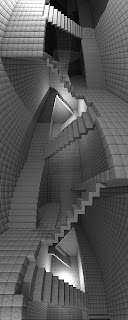
The target is the representation in 3D of the picture "House Of Stairs" of M.C.Escher. I focused the representation of walls and stairs. The strange animals and the doors are missing.

The results are these, in black and white and in color:

In the color version I have simply used blackbody illuminants with temperatures of 3000, 4000, 5000 and 7000 Kelvin.

In order to make the renders we have to do this. It's necessary to model the scenery in such a way so the dimensions fit using whole units (fitting into a grid). So we make sure that all walls, walkways and stairs have similar widths. With any CAD program it's possible to model the scenery looking the original drawing. The objects at this point have box geometry.



Because the rendering of boxes is too dull we have to add some effects. One of those has to emulate the round shape of a stone. In order to achieve that we can use textures or 3D models. In this case I preferred using 3D models to achieve more quality. Accomplishing this is simple. We cubicate the scene with the same resolution of the design grid. Now we have a set of voxels. Each voxel is replaced by a rounded cube mesh shape. The only problem is the amount of data and so the high processing time.



Later we apply a material to the surface. For that is used a composite material. The material is composed by one control map and two data maps. The control material is used to decide the amount of blending between the data materials. It's similar to an alpha blending. For the control map I have used a binary threshold discretized Perlin noise function. In the high part I have assigned one kind of bumpmap and in the lowest part another kind. So, two bumpmaps of controllable independent characteristics are obtained. Now we simply apply a greater scale factor and noise to one to look like holes in stone, while applying a smoother noise to the other. With only one bumpmap would have achieved a smoothed and polished stone effect with some holes. We don't want it.



Finally to render it's used a cylindrical camera to emulate the curved effect of "The House of Stairs". With a little wise we can place the camera more or less the same position where Escher sat it.

Hoy voy a mostrar una serie de renders que aunque no están totalmente acabados me gustaría enseñar.
El objetivo es la representación en 3D del dibujo "Casa de Escaleras" de M.C.Escher. Me he centrado en la representación de los muros y las escaleras. Faltan los animales extraños y las puertas.

Los resultados son los siguientes, en blanco y negro y en color:

Para la versión en color simplemente he utilizado iluminantes de cuerpo negro a temperaturas de 3000, 4000, 5000 y 7000 Kelvin.

Para realizar los renders se parte de lo siguiente. Es necesario modelar un escenario de tal forma que las medidas se ajusten a unidades enteras (ajustado a un grid). Así nos aseguramos que todos los muros, pasarelas y escaleras tienen anchuras similares.
Con cualquier programa de CAD se puede modelar el escenario fijándose bien en el dibujo original. Los objetos en este punto tienen una geometría de cajas.



Cómo la renderización de cajas es muy sosa se han de añadir algunos efectos. Uno tiene que poder emular la forma redondeada de la piedra. Para ello se pueden utilizar texturas o modelos 3D. En este caso he preferido utilizar modelos 3D para obtener una mejor calidad. La realización de esto es sencilla. Se cubica la escena a la misma resolución que la del grid de diseño. Ahora tenemos un conjunto de vóxeles. Cada vóxel se sustituye por una malla en forma de cubo con bordes redondeados. El único problema de esto es la cantidad de datos y por lo tanto el tiempo elevado de proceso.



Posteriormente se aplica un material a la superficie. Para ello se utiliza un material compuesto. El material se compone de un mapa de control y dos de datos. El mapa de control se utiliza para determinar la cantidad de mezcla de los materiales de datos. Similar a una mezcla alfa. Para el mapa de control he utilizado ruido de Perlin discretizado por un umbral binario. A la parte superior le aplico un tipo de bumpmap y a la parte inferior otro. Por lo que se obtienen dos bumpmaps de características controlables independientemente. Ahora simplemente se aplica un mayor factor de escala y ruido a uno para que parezcan agujeros en piedra, mientras que al otro un ruido mucho más suave. Con un solo mapa de bumpmap se habría conseguido un efecto de pierda lisa y pulida con algunos agujeros, cosa que no se quiere.



Finalmente para la renderización se utiliza una cámara cilíndrica para emular el efecto de "La Casa de las Escaleras". Con un poco de tino se puede situar la cámara más o menos en la misma posición de dónde la situó Escher.

Spatial Labyrinths

English    Spanish

Today I'm going to show a set of renders that I did some time ago. The general idea is to make a spatial maze.

That is, one that allows movements upwards and downwards as well as forward, backward, right and left. The movements that a player can do are in any spatial axis. In this case, Theseus has to know how to climb well.

One simple is this one:

In this one we see a tridimensional labyrinth bounded by the surface of a cube.

The procedure to accomplish this renders is not complex.

• We start from a tridimensional shape. Then it's discretized in voxels marking as active the ones that are partially or totally included in the volume defined by the surface of the figure.
• Now we are going to discard the non active voxels and we work with the ones that intersect or are included inside the volume.
• We start from a random voxel and we move in a random direction, marking as visited the currant voxel.
• As we move through the voxels we can find a visited voxel in the chosen direction. In this case we chose another direction.
• In the case that there are not any available directions we move backwards and we chose another direction.
  
• The algorithm ends when all the nodes (voxels) have been visited.

This algorithm allows a unique path from one point of the labyrinth to another. Obviously if we set two poins, one as starting and another one as ending, there will be a unique path between both, and then any other bifurcation that moves away from the path will bring us to a dead end.

Other views of the cube:

It's possible to use other figures as a "mould" of the labyrinth.

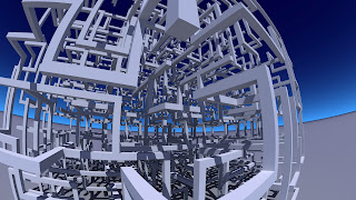
Here we can see a sphere:





And with a spherical camera:





The Utah teapot:



and a some renderings of a lying woman:

Hoy voy a mostrar una serie de renders que hice hace poco. La idea general es realizar un laberinto espacial.

Esto es, que permita movimentos hacia arriba y hacia abajo además de adelante, atrás, derecha e izquierda. Los movimientos que puede efectuar un jugador serían en cualquier eje espacial. En este caso Teseo deberá saber escalar bien.

Un ejemplo es el siguiente:

En éste vemos un laberinto tridimensional acotado por la superficie de un cubo.

Para realizar estos renders el procedimiento no es complicado.

• Se parte de una figura tridimensional.Se discretiza en vóxeles marcando como vóxel activo un voxel que está parcial o totalmente incluido en el volumen definido por la superficie de la figura.
• A partir de ahora vamos a descartar los vóxeles no activos y trabajamos con aquellos que intersectan o están incluidos en el volumen.
• Partimos de un vóxel aleatorio y nos movemos en una dirección aleatoria, marcando éste vóxel como visitado.
• A medida que avanzamos nos podemos encontrar con un voxel ya visitado en la dirección elegida. En este caso elegimos otra dirección.
• En el caso de no existan direcciones disponibles, damos un paso hacia atrás (backtracking) y repetimos el proceso.
• El algoritmo finaliza cuando hemos visitado todos los nodos activos.

Este algoritmo permite un camino único desde un punto del laberinto hasta cualquier otro. Obviamente si fijamos dos puntos, uno de comienzo y otro de fin, existirá un camino único, y por lo tanto cualquier bifurcación que se separe de dicha ruta llevará a un extremo sin salida.

Otras vistas del cubo:

Se pueden utilizar otras figuras como "molde" del laberinto

Aquí vemos una esfera:





Y con una cámara esférica:





La tetera de Utah:



Y unas representaciones de una mujer tumbada: